Mahout "Samsara" book prerequisites

Q: "... Any tips on prerequisite reading?"

A: To quote the preface of the book:

"Some material assumes an undergraduate level understanding of calculus and on occasion multivariate calculus. The examples are given in Scala and assume familiarity with basic Scala terminology and a minimal notion of functional programming."

Let's elaborate.

There are two sides: the technology side and the math side.

For the technology side, the reader would benefit from some Scala fluency and functional programming. Public Scala material presented on http://scala-lang.org/ gets one a long way, plus of course there's always a longer book by Martin Odersky, et. al., "Programming in Scala".

For the math side, note that we do not explain math. We do not ask ourselves the question "Can I understand it [why it works]?", but rather we ask the question "Can I try it?". A lot of practical research is working exactly just like that -- by asking ourselves the question "What if I try this or that?". So it is not so much about math but rather about math notations, which are for our purposes is pseudocode that we turn into code. Math notations are sufficiently explained in the section A.2; if you have a concrete question beyond what is there, please ask -- we will try to answer.

Beyond notations, it would help to be familiar with the undergraduate level of linear algebra and calculus (after all, we are trying to deal with applied machine learning).

For linear algebra, a good reference is the textbook by Gilbert Strang, "Introduction to Linear Algebra". Algorithms we illustrate at times rely on working knowledge of singular value decomposition (SVD), eigendecomposition, Cholesky decomposition and QR decomposition, as well as Four Fundamental subspaces.

It has been some time since I studied multivariate calculus, so I am not quite sure what the best text is on it these days. I have the "Multivariate Calculus" book by Larson Edwards, which is pretty thorough in my opinion. We do not need all of it though; our book examples touch on very few notions of multivariate calculus -- partial derivatives, gradient, Hessian matrix. As a refresher, perhaps even reading Wikipedia articles on these issues is enough.

Of course when one works on a particular algorithm, she or he needs to read the publication containing the algorithm formulation. That is one of the things that we are trying to demonstrate: how to read and implement algorithm formulations using Mahout "Samsara". We give references to the algorithm publications as appropriate, throughout the book.

-DL

Mahout "Samsara" Book Is Out

After many months of work, our book is finally out.

Here is our formal announcement:


We are happy to announce that Mahout Samsara is finally documented in print. The book title is “Apache Mahout: Beyond MapReduce.”

Similar to other books on computer science or languages such as R, Python, or C++, the authors are hoping to put the reader on the path of designing and creating his or her own algorithms. Also included are tutorials and practical usage information about newer Mahout algorithms.

The emphasis is on Machine Learning algorithm design aspects in the context of Apache Mahout “Samsara” releases (0.10, 0.11). If there were another suitable name for this book, it might be “Beyond the Black Box”: the discussions go beyond the scope of just the Mahout environment or Mahout algorithms and touch on more general concepts for devising algorithms in the context of massive inputs and computations, using Mahout Samsara as a semantical implementation medium for the solutions.

Mahout “Samsara” currently targets H2O, Apache Flink and Apache Spark as backend execution options. As work on the Apache Flink backend is still in progress, all examples, while being execution engine agnostic (with one intended exception), are set up to run with the Apache Spark backend.

This work has been greatly helped by valuable reviews and ideas from other Mahout committers, contributors, and industry professionals, as indicated in the “Acknowledgments” section of the preface (Thank you!).

This book does not discuss legacy MapReduce-based algorithms.

Thank you for using Mahout!

Dmitriy Lyubimov (@dlieuOfTwit)
Andrew Palumbo (@andy_palumbo)

Technical info:

There are two editions of the book: a black and white paperback and a full color Kindle textbook.

The Kindle textbook completely preserves the layout of the paperback edition. It is enrolled in the Amazon “Matchbook” program (free with the purchase of a print copy when ordered via Amazon.com).

The paperback edition has been optimized specifically for a black-and-white print. The format is 7x10in. (a common textbook size).

Code examples are available on GitHub.

Where:

Amazon.

Update: Createspace now has closed their online book store it seems, and just redirects to Amazon, so we cannot seem to set discounts any longer thru them.
In the US a paperback-only copy can also be purchased here with a 25% off code QLZ8DLPL.

Antother update: the electronic copy can now be obtained here at no cost. Of course Amazon is still the way to have the paper version or on Kindle, but they are no longer the exclusive distributor. Please note that the copyright applies (no redistribution beyond this blog; no reproduction beyond fair use). If you want to link to the book, we will appreciate if you link this blog post (https://weatheringthrutechdays.blogspot.com/2016/02/mahout-samsara-book-is-out.html), rather than the direct download. Thank you.

---

Post Scriptum 

Thank you for reading!

See also: Book prerequisites, Errata updates

Mahout 0.10.x: first Mahout release as a programming environment

Mahout 0.10.x is coming. It is a new generation of Mahout that entirely re-thinks philosophy of previous Mahout line of releases. 

First, and foremost, to state the obvious, Mahout abandons MapReduce based algorithms. We still support them (and they are now moved to mahout-mr artifact). But we do not create any new ones. 

Second, we shift the focus from being a collection of things to being a programming environment, as it stands, for Scala.

Third, we support different distributed engines, aka "backs". As it stands, we run on Spark and H20, but hope to add Apache Flink translation as well, provided we get help there.

Many people are coming with obvious question: so how it is different from stuff like MLLib? Here, I'll try to emphasize key philosophical points of this work. 

1. We want to help people to create their own math, as opposed to just taking and plugging in an off-the-shelf black-box solution. 

Indeed, having a fairly well-adjusted and complicated black box solutions is a good thing. People spent quite a bit of time researching and optimizing them. 

Problem is, very often off-the-shelf is just not enough. We want to customize and build our own models, our own features, our own specific rules and ensembles. And we want to do it quickly and try it now.

Let's look at some intentionally simple examples. Suppose we want to compute a column-wise variances on a matrix. For that we are going to use simple formula

\[
\mathrm{var}\left(x\right)=\mathbb{E}\left(x^{2}\right)-\left[\mathbb{E}\left(x\right)\right]^{2}
\]

applied column-wise on our big, distributed matrix $\mathbf{X}$. Here is how it is going to look in new Mahout enviornment: 

val mu = X colMeans
val variance = (X * X colMeans) -= mu * mu

That's it. All in fully distributed fashion. On Spark or H20. 

Let's take on a little bit more complicated case. What if we want to compute n-dimensional column-wise covariance matrix of the dataset X? 

Assuming that

\[
\boldsymbol{x}_{i}\triangleq\mathbf{X}_{i*},
\]

i.e. every row is a point in the dataset, we can use multivariate generalization of the previous formula:

\[\mathrm{cov}\left(\mathbf{X}\right)=\mathbb{E}\left(\boldsymbol{xx}^{\top}\right)-\boldsymbol{\mu\mu}^{\top},\]

where

\[\boldsymbol{\mu}=\mathbb{E}\left(\boldsymbol{x}\right).\]

Here is the Mahout code for that formula: 

val mu = X.colMeans()
val mxCov = (X.t %*% X).collect /= X.nrow -= (mu cross mu)

This code is actually a so called "thin" procedure, i.e. the one that assumes that while the  $m\times n$ input matrix $\mathbf{X}$ is too big to be an in-core matrix, the $n\times n$ covariance matrix   will fit into memory in one chunk. In other words, it assumes $n\ll m$. The code for "wide" distributed covariance computation needs couple more lines but is just as readable.

So, what is the difference between Mahout 0.10.x and MLLib? Well, what is the difference between R package and R? What is the difference between libsvm and Julia? What is difference between Weka and Python? And how to think about it -- R for Spark? Hive for math? Choose your poison.

Bottom line, we want to help you create your own math at scale. (And hopefully, come back to us and share it with us).

2. We want to simplify dialect learning. We actually build the environment in image of R. Initially, we also had DSL dialect (enabled via separate import) for Matlab, but unfortunately Scala operator limits do not make it possible to implement entire Matlab operator set verbatim, so this work received much less attention, and instead, we focused on R side of things.

What it means is it should be easily readable by R programmers. E.g. A %*% B is matrix multiplication, A * B is elementwise Hadamard product, methods like colMeans, colSums are following R naming for those.

Among other things, arguably, math written in R-like fashion is easier to understand and maintain than the same things written in other basic procedural or functional environments.

3. Environment is backend-agnostic. Indeed, Mahout is not positioning itself as Spark-specific. You can think of it that way if you use Spark, but if you use H20, you could think of it as H2o-specifc (or, hopefully, "Apache Flink-specifc" in the future) just as easily.

All the examples above are not containing a single Spark (or h20) imported dependency. They are written once but run on any of supported backs.

Not all things can be written with the subset of back-independent techniques of course, more on that below. But quite a few can -- and the majority can leverage at least some as the backbone. E.g. imagine that dataset $\mathbf{X}$ above is result of embarrassingly parallel statistical Monte Carlo technique (which is also backend-independent). And just like that we perhaps get a backend-agnostic Gibbs sampler.

4. "Vs. mllib" is a false dilemma. Mahout is not taking away any capabilities of the backend. Instead, one can think of it as an "add-on" over e.g. Spark and all its technologies. (same for h2o).

Indeed, it is quite common to expect that just Algebra and stats are not enough to make the ends meet. In Spark's case, one can embed algebraic pipelines by importing Spark-specific capabilities. Import MLLib and all the goodies are here. Import GraphX and all the goodies are here as well. Import DataFrame(or SchemaRDD) and use language-integrated QL. And so on.

I personally use one mllib method as a part of my program along with Mahout algebra. On the same Spark context session as the Mahout Algebra session. No problem here at all.

5. Mahout environment is more than just a Scala DSL. Behind the scenes, there is an algebraic optimizer that creates logical and physical execution plans, just like in a database.

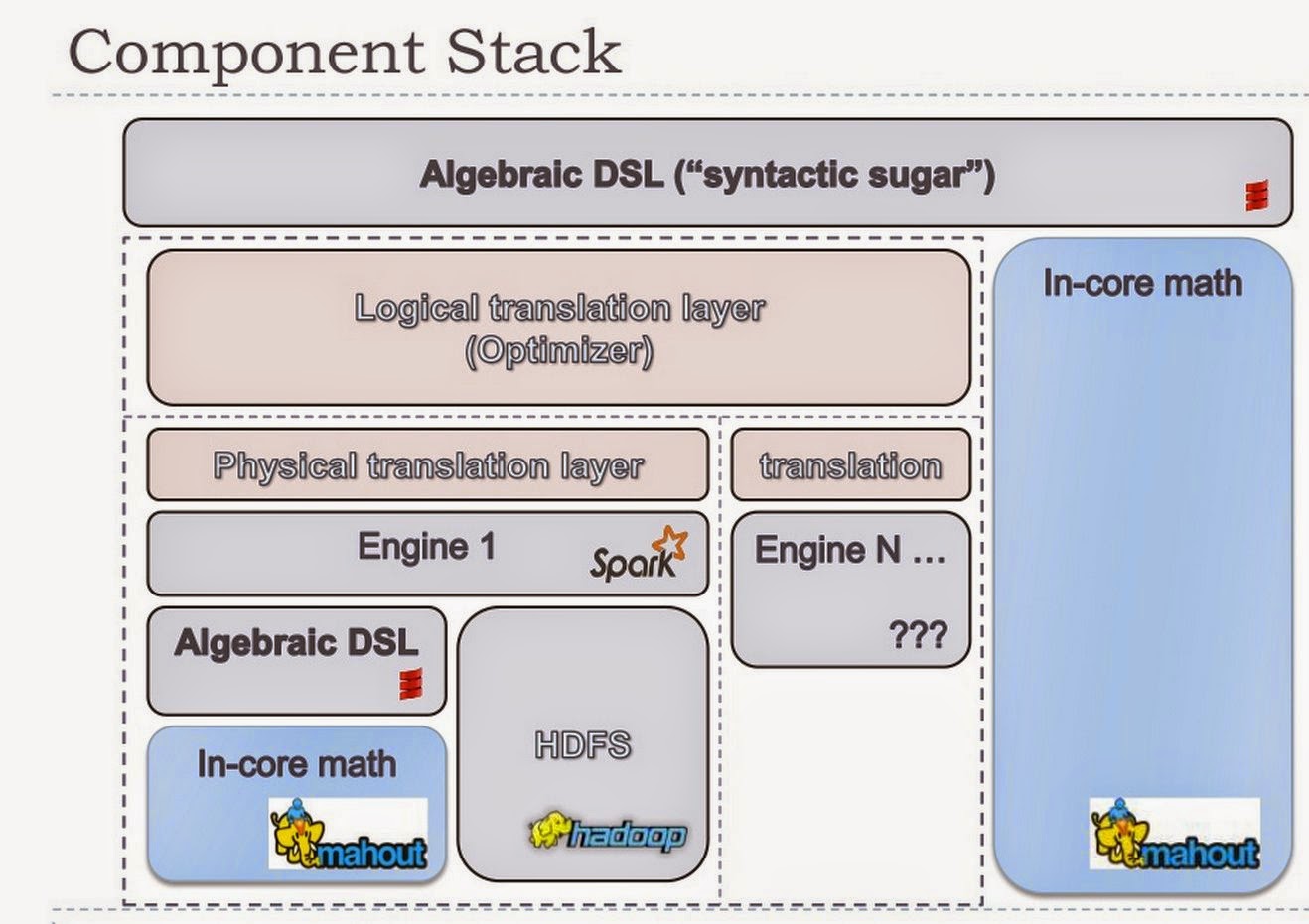Algebraic Optimizer Stack

For example, we can understand that a thing like 

dlog(X * X + 1).t %*% dlog(X * X + 1) 

 is in fact (in simplified physical operator pseudo code)

self_square(X.map(x => log(x * x + 1)).

6. Off-the-shelf methods. Of course we want to provide off-the-shelf experience too. Logical thing here is to go with stuff that complements, but not repeats other off-the-shelf things available. Refer to the Mahout site what's in and what's in progress.

But even use of off-the-shelf methods should be easily composable via programming environment and scripting.

Future plans. Work is by no means complete. In fact, it probably just started.

In more or less near future we plan to extend statistical side of things of the environment quite a bit.

We plan to work on performance issues, especially for in-core performance of the algebraic API.

We want to port most of MR stuff to run in the new environment, preferably in a completely backend-agnostic way (and where it is not plausible, we would isolate and add strategies for individual backs for the pieces that are not agnostic).

We plan to add some must-have off-the-shelf techniques such as hyperparameter search.

And of course, there are always bugs and bug fixes.

Longer term, we think it'd be awesome to add some visualization techniques similar to ggplot2 in R, but we don't have capacity to develop anything similar from the ground up, and we are not yet sure what might be integrated in easily and which also works well with JVM based code. Any ideas are appreciated.

#Mahout 0.7 has more usable PCA workflow now

Now that Mahout 0.7 has been released, it is probably appropriate to say a word with respect to my contribution, MAHOUT-817, that enables (afaik, for the first time) for Mahout to have a PCA workflow. (Well, in all fairness, I wasn't alone contributor there. Many thanks to Raphael Cendrillon for contributing the mean computation map-reduce step).

It is based on SSVD method that computes mathematical SVD in a distributed way. Generally, there's no problem using brute-force PCA approach that involves mean subtraction and then running SVD on the result.

The only time when the wrench is thrown into that engine is when original PCA input matrix is sufficiently sparse. Making mean subtraction is going to transform input matrix into a dense matrix, potentially increasing number of non-zero elements (and hence, flops needed to complete matrix operations during SVD computation) many times.

As it is true for many Mahout methods, SSVD actually takes a big view of the world with all its details and produces a more condensed analytic view of the world. So the natural thinking to deal with that is, ok, can we just run an SVD first on the sparse input and fix the smaller condensed view at its smallest incarnations later so that creates summary equivalent to that with mean subtraction?

Here is the quick write-up that shows how the math for that neat trick has worked out in Mahout.



Also, a high-level overview and practical usage of this approach is given : https://cwiki.apache.org/confluence/display/MAHOUT/Stochastic+Singular+Value+Decomposition.

#Mahout #MapReduce #SSVD version gets power iterations, fixes

I have been working on MAHOUT-796 this week (current work is in https://github.com/dlyubimov/mahout-commits/tree/MAHOUT-796).


Nathan Halko pointed to me that power iterations in practice improve precision and reduce noise.


After a little discussion, that's the route we went :

 Original formula 

\[\mathbf{Q}=\mbox{qr}\left[\left(\mathbf{AA^{\top}}\right)^q\mathbf{A}\boldsymbol{\Omega}\right].\mathbf{Q},\]

\[\mathbf{B}=\mathbf{Q}^{\top}\mathbf{A}.\]

Modified version 

\[\mathbf{Y}=\mathbf{A}\boldsymbol{\Omega},\]

\[\mathbf{B}_{0}=\left[\mbox{qr}\left(\mathbf{Y}\right).\mathbf{Q}\right]^{\top}\mathbf{A},\]

\[\mathbf{B}_{i}=\left[\mbox{qr}\left(\mathbf{AB}_{i-1}^{\top}\right).\mathbf{Q}\right]^{\top}\mathbf{A},\, i\in\left[1..q\right].\]

Notation \(\mbox{qr}\left(\cdot\right).\mathbf{Q}\) means "compute QR decomposition of the argument and retain Q as a result". 

Current combination of QJob and BtJob is essentially producing \(\mathbf{B}_{0}^{\top}=\mathbf{A}^{\top}\mbox{qr}\left(\mathbf{A}\boldsymbol{\Omega}\right).\mathbf{Q}\). Intermediate QJob results are QR blocks, not a final Q, so QJob is not terribly meaningful without BtJob.

The task boils down to figuring out alternative pipeline modifications necessary to produce \(\mathbf{B}_{i}^{\top}\). After that, algorithm proceeds as before with assumption of \[\mathbf{B}\equiv\mathbf{B}_{q}.\] 

The existing processing will be equivalent to \({q}=0\). 

\(\mathbf{B}_{i}\) pipeline (some new code)

\(\mathbf{B}_{i}\) pipeline produces \[\mathbf{B}_{i}^{\top}=\mathbf{A}^{\top}\mbox{qr}\left(\mathbf{A}\mathbf{B}^{\top}\right).\mathbf{Q}.\]

this is very similar to \(\mathbf{B}_{0}\) pipeline with specfics being full multiplication of \(\mathbf{A}\mathbf{B}^{\top}\) in the first job and first pass qr pushdown to the reducer of the first job:

• map1 : \(\mathbf{A}\mathbf{B}^{\top}\) outer products are produced 
• combiner1 : presumming outer products of \(\mathbf{A}\mathbf{B}^{\top}\).
• reducer1 finalizes summing up outer products of \(\mathbf{A}\mathbf{B}^{\top}\) and starts \(\mbox{qrFirstPass}\left(\mathbf{A}\mathbf{B}^{\top}\right)\to\mbox{qr blocks}\). (partitioning must be done by A block # it seems).
• mapper2, combiner2, reducer2 proceed exactly as mapper2, combiner2, reducer2 in B pipeline and output final \(\mathbf{B}_{i}^{\top}\) with blocks corresponding to initial splits of A input.

Thus, this pipeline is 2 MR jobs with 2 sorts (map1 + combiner1 + shuffle and sort + reducer1 + map2 + combiner2 + shuffle and sort + reducer2).

Integration of Cholesky trick route for computing power iterations 

Ted Dunning pointed out that the whole B pipeline could avoid QR step.

When power iterations are concened, note that whatever route is chosen to calculate \(\mathbf{B}_{i}=g\left(\mathbf{Y}_{i}\right)\), mathematically it should still be valid \(\forall i\in\left[0..q\right]\) for as long as we assume 

\[\mathbf{Y}_{0}=\mathbf{A}\boldsymbol{\Omega}, i=0;\]

\[\mathbf{Y}_{i}=\mathbf{A}\mathbf{B}_{i-1}^{\top}, i>{0}.\] 

So, if Cholesky trick allows to produce \(\mathbf{B}_{0}\) efficiently, I see no reason why it could not be applied to producing the \(\mathbf{B}_{i}\).

I will be pursuing MR option of running Cholesky decompositon of \(\mathbf{Y}^{\top}\mathbf{Y}\) in MAHOUT-797.

If that holds, then power iterations with Cholesky decomposition will likely be similar. 

\(\mathbf{LL}^{\top}=\mathbf{Y}^{\top}\mathbf{Y}=\mathbf{R}^{\top}\mathbf{R}\Rightarrow\) we know how to compute \(\mathbf{R}\);

\[\mathbf{B}_{i}=\left(\mathbf{R}^{-1}\right)^{\top}\mathbf{Y_{i}}^{\top}\mathbf{A};\]

\[\mathbf{Y}_{0}=\mathbf{A}\boldsymbol{\Omega}, i=0;\]

\[\mathbf{Y}_{i}=\mathbf{A}\mathbf{B}_{i-1}^{\top}, i>{0}.\]

Tests

Tests with local MR QR-based solver seem to be encouraging. There's clear improvement on precision. 

With surrogate random input with predefined singular values 10,4,1,(0.1...), toy input 2000x1000 and k=3,p=10 I seem to be getting improvement after just one additional power iteration:

q=0: 

--SSVD solver singular values:
svs: 9.998472 3.993542 0.990456 0.100000 0.100000 0.100000 0.100000 0.100000 0.100000 0.100000 0.100000 0.100000 0.100000

q=1: (+2 more MR sequential steps):
--SSVD solver singular values:
svs: 10.000000 4.000000 0.999999 0.100000 0.100000 0.100000 0.100000 0.100000 0.100000 0.100000 0.100000 0.100000 0.100000

After some tests and cleanup, I guess it is going to become a commit really soon.

Bug fixes

In addition to all this, MAHOUT-796 branch gets a lot of bug fixes (in particular, better handling sparse inputs which seemed to have still been broken in current version).

Streaming QR decomposition for MapReduce part III: Collecting Q by Induction

In Part II, as a part of bottom-up divide-and-conquer parallelization strategy, one problem emerged that we need to solve at every node of bottom-up tree:

$$\left(\begin{matrix}\left(\begin{matrix}\mathbf{Q}_{1}\\\mathbf{Q}_{2}\\\vdots\\\mathbf{Q}\end{matrix}\right)\mathbf{R}_{1}\\\left(\begin{matrix}\mathbf{Q}\\\mathbf{Q}\\\vdots\\\mathbf{Q}\end{matrix}\right)\mathbf{R}_{2}\\\vdots\\\left(\begin{matrix}\mathbf{Q}\\\mathbf{Q}\\\vdots\\\mathbf{Q}_{z}\end{matrix}\right)\mathbf{R}_{n}\end{matrix}\right)=\left(\begin{matrix}\mathbf{\hat{Q}}\\\mathbf{\hat{Q}}\\\vdots\\\mathbf{\hat{Q}}\end{matrix}\right)\mathbf{\hat{R}}$$        (1)       

Let's simplify the problem for a moment (as it turns out, vertical blocking of Q is trivial as they are always produced by application of column-wise Givens operations which we can 'replay' on any Q block).

$$\left(\begin{matrix}\mathbf{Q}_{1}\mathbf{R}_{1}\\\mathbf{Q}_{2}\mathbf{R}_{2}\\\cdots\\\mathbf{Q}_{z}\mathbf{R}_{z}\end{matrix}\right)\Rightarrow\left(\begin{matrix}\mathbf{\hat{Q}}_{1}\\\mathbf{\hat{Q}}_{2}\\\cdots\\\mathbf{\hat{Q}}_{z}\end{matrix}\right)\hat{\mathbf{R}}$$     (2)

Also let's decompose standard Givens QR operation in to two:

1) producing Givens transformation sequence on some input $m\times n$, $m>n$  A as $$\left(\mathbf{G}_{1},\mathbf{G}_{2}...\mathbf{G}_{k}\right)=\mathrm{givens\_qr}\left(\mathbf{A}\right)$$.  I will denote product of all Givens operations obtained this way as $$\prod_{i}\mathbf{G}_{i}\equiv\prod\mathrm{givens\_qr}\left(\mathbf{A}\right)$$.

2) Applying product of Givens operations on input produces already familiar result
\[\left(\prod_{i}\mathbf{G}_{i}\right)^{\top}\mathbf{A}=\left(\begin{matrix}\mathbf{R}\\\mathbf{Z}\end{matrix}\right)\]

from which it follows that thin QR's R can be written as
\[\mathbf{R}=\left[\left(\prod_{i}\mathbf{G}_{i}\right)^{\top}\mathbf{A}\right]\left(1:n,:\right)=\left[\left(\prod\mathrm{givens\_qr}\left(\mathbf{A}\right)\right)^{\top}\mathbf{A}\right]\left(1:n,:\right)\]
using Golub/Van Loan's block notation.

(Golub/Van Loan's block notation in form of A(a₁:a₂, b₁:b₂) means "crop of a matrix A, rows a₁ to a₂ and columns b₁ to b₂". For half- and full-open intervals the bounds are just omitted).

'Thick' Q is produced by $$\mathbf{I}\left(\prod_{i}\mathbf{G}_{i}\right)$$ and hence 'thin Q' is
\[\mathbf{Q}=\left[\mathbf{I}\left(\prod_{i}\mathbf{G}_{i}\right)\right]\left(:,1:n\right)=\left[\mathbf{I}\left(\prod_{i}\mathrm{givens\_qr}\left(\mathbf{A}\right)\right)\right]\left(:,1:n\right),\mathbf{\,\, I}\in\mathbb{R}^{m\times m}.\]

Now that we laid out all notations, let's get to the gist. As I mentioned before, I continue building algorithm by induction. Let's consider case (2) for $$z=2$$. Then it can be demonstrated that the following is the solution as it is equivalent to full Givens QR with a rearranged but legitimate order of Givens operations:

$$\mathbf{\hat{R}}=\left\{\left[\prod\mathrm{givens\_qr}\left(\begin{matrix}\mathbf{R}_{1}\\\mathbf{R}_{2}\end{matrix}\right)\right]^{\top}\cdot\left(\begin{matrix}\mathbf{R}_{1}\\\mathbf{R}_{2}\end{matrix}\right)\right\} \left(1:n,:\right)$$,

$$\mathbf{\hat{Q}=}\left[\left(\begin{matrix}\mathbf{Q}_{1} & \mathbf{Z}\\\mathbf{Z} & \mathbf{Q}_{2}\end{matrix}\right)\cdot\prod_{i}\mathrm{givens\_qr}\left(\begin{matrix}\mathbf{R}_{1}\\\mathbf{R}_{2}\end{matrix}\right)\right]\left(:,1:n\right)$$.

Let's denote function of 2-block computation of $$\mathbf{\hat{R}}$$ as 

$$\mathrm{rhat}\left(\mathbf{R}_{i},\mathbf{R}_{j}\right)=\left\{\left[\prod\mathrm{givens\_qr}\left(\begin{matrix}\mathbf{R}_{i}\\\mathbf{R}_{j}\end{matrix}\right)\right]^{\top}\cdot\left(\begin{matrix}\mathbf{R}_{i}\\\mathbf{R}_{j}\end{matrix}\right)\right\} \left(1:n,:\right)$$.

Still working on the trivial case of induction: Now note that since Givens operations for calculation of $$\mathbf{\hat{Q}}$$ are applied pairwise to the columns of the accumulator matrix, i.e. independently for each row, we can split computation of $$\mathbf{\hat{Q}}$$ and apply it to any combination of vertical blocks of $$\left(\begin{matrix}\mathbf{Q}_{1} & \mathbf{Z}\\\mathbf{Z} & \mathbf{Q}_{2}\end{matrix}\right)$$. Let's say we decide to split it into 2 blocks with as many rows as in Q₁ and Q₂ and get back to block-wise formulas sought for solution of (2):

$$\mathbf{\hat{Q}_{1}=}\left[\left(\begin{matrix}\mathbf{Q}_{1} & \mathbf{Z}\end{matrix}\right)\cdot\prod_{i}\mathrm{givens\_qr}\left(\begin{matrix}\mathbf{R}_{1}\\\mathbf{R}_{2}\end{matrix}\right)\right]\left(:,1:n\right),$$

$$\mathbf{\hat{Q}_{2}=}\left[\left(\begin{matrix}\mathbf{Z} & \mathbf{Q}_{2}\end{matrix}\right)\cdot\prod_{i}\mathrm{givens\_qr}\left(\begin{matrix}\mathbf{R}_{1}\\\mathbf{R}_{2}\end{matrix}\right)\right]\left(:,1:n\right).$$      (3)

Let's denote those transformations in more general form as 

$$\mathrm{qhat\_down}\left(\mathbf{Q}_{i},\mathbf{R}_{i},\mathbf{R}_{j}\right)=\left[\left(\begin{matrix}\mathbf{Q}_{i} & \mathbf{Z}\end{matrix}\right)\cdot\prod\mathrm{givens\_qr}\left(\begin{matrix}\mathbf{R}_{i}\\\mathbf{R}_{j}\end{matrix}\right)\right]\left(:,1:n\right)$$

and

$$\mathrm{qhat\_up}\left(\mathbf{Q}_{i},\mathbf{R}_{i},\mathbf{R}_{j}\right)=\left[\left(\begin{matrix}\mathbf{Z} & \mathbf{Q}_{i}\end{matrix}\right)\cdot\prod\mathrm{givens\_qr}\left(\begin{matrix}\mathbf{R}_{j}\\\mathbf{R}_{i}\end{matrix}\right)\right]\left(:,1:n\right)$$

then we can rewrite (3) as

$$\mathbf{\hat{Q}}=\left(\begin{matrix}\mathbf{\hat{Q}}_{1}\\\mathbf{\hat{Q}}_{2}\end{matrix}\right)=\left(\begin{matrix}\mathrm{qhat\_down}\left(\mathbf{Q}_{1},\mathbf{R}_{1},\mathbf{R}_{2}\right)\\\mathrm{qhat\_up}\left(\mathbf{Q}_{2},\mathbf{R}_{2},\mathbf{R}_{1}\right)\end{matrix}\right)$$,

$$\mathbf{\hat{R}}=\mathrm{rhat}\left(\begin{matrix}\mathbf{R}_{1}\\\mathbf{R}_{2}\end{matrix}\right)$$

This is our solution for (2) of trivial case (z=2).

I will show solution for z=3 and then just will give the final solution without a proof.

Case z=3:

Note that functions qhat_up() and qhat_down() also implicitly produce intermediate rhat() products during their computation, so we want to 'enhance' them to capture that rhat() result as well. We will denote 'evolving' intermediate results Q and R as a sequence $$\left(\mathbf{\tilde{Q}},\mathbf{\tilde{R}}\right)$$:

$$\mathrm{qrhat\_down}\left(\mathbf{Q}_{i},\mathbf{R}_{i},\mathbf{R}_{j}\right)=\left(\mathbf{\tilde{Q}},\mathbf{\tilde{R}}\right)=\left(\mathrm{qhat\_down}\left(\mathbf{Q}_{i},\mathbf{R}_{i},\mathbf{R}_{j}\right),\mathrm{rhat}\left(\mathbf{R}_{i},\mathbf{R}_{j}\right)\right)$$,

$$\mathrm{qrhat\_up}\left(\mathbf{Q}_{i},\mathbf{R}_{i},\mathbf{R}_{j}\right)=\left(\mathbf{\tilde{Q}},\mathbf{\tilde{R}}\right)=\left(\mathrm{qhat\_up}\left(\mathbf{Q}_{i},\mathbf{R}_{i},\mathbf{R}_{j}\right),\mathrm{rhat}\left(\mathbf{R}_{j},\mathbf{R}_{i}\right)\right)$$.

Then, using those notations, we can write solution for (2) z=3 as

$$\mathbf{\hat{Q}}=\left(\begin{matrix}\mathbf{\hat{Q}}_{1}\\\mathbf{\hat{Q}}_{2}\\\mathbf{\hat{Q}}_{3}\end{matrix}\right)=\left(\begin{matrix}\mathrm{qrhat\_down}\left(\mathrm{qrhat\_down}\left(\mathbf{Q}_{1},\mathbf{R}_{1},\mathbf{R}_{2}\right),\mathbf{R}_{3}\right).\mathbf{\tilde{Q}}\\\mathrm{qrhat\_down}\left(\mathrm{qrhat\_up}\left(\mathbf{Q}_{2},\mathbf{R}_{2},\mathbf{R}_{1}\right),\mathbf{R}_{3}\right).\mathbf{\tilde{Q}}\\\mathrm{qrhat\_up}\left(\mathbf{Q}_{3},\mathbf{R}_{3},\mathrm{rhat}\left(\mathbf{R}_{1},\mathbf{R}_{2}\right)\right).\mathbf{\tilde{Q}}\end{matrix}\right)$$.

Note that algorithm for computing $$\mathbf{\hat{Q}}_i$$ requires input of Q_i, iterator[(R₁,R₂...R_z)].

General solution for (2) for any z is built by induction as the following algorithm:

This algorithm is still sub-efficient as for the entire matrix (2) it computes more rhat() operations than needed, and can be optimized to reduce those operations when considering final solution for (1),  but that's probably too many details for this post for now. Actual details are found in code and my working notes.

Finally, a word about how to transform solution for (2) into a solution for (1).

We can rewrite indexes in (1) as

$$\left(\begin{matrix}\left(\begin{matrix}\mathbf{Q}_{1}\\\mathbf{Q}_{2}\\\cdots\\\mathbf{Q}\end{matrix}\right)\mathbf{R}_{1}\\\left(\begin{matrix}\mathbf{Q}\\\mathbf{Q}\\\cdots\\\mathbf{Q}\end{matrix}\right)\mathbf{R}_{2}\\\cdots\\\left(\begin{matrix}\mathbf{Q}\\\mathbf{Q}\\\cdots\\\mathbf{Q}_{z}\end{matrix}\right)\mathbf{R}_{n}\end{matrix}\right)\equiv\left(\begin{matrix}\left(\begin{matrix}\mathbf{Q}_{11}\\\mathbf{Q}_{12}\\\cdots\\\mathbf{Q}_{1k}\end{matrix}\right)\mathbf{R}_{1}\\\left(\begin{matrix}\mathbf{Q}_{21}\\\mathbf{Q}_{22}\\\cdots\\\mathbf{Q}_{2k}\end{matrix}\right)\mathbf{R}_{2}\\\cdots\\\left(\begin{matrix}\mathbf{Q}_{n1}\\\mathbf{Q}_{n2}\\\cdots\\\mathbf{Q}_{nk}\end{matrix}\right)\mathbf{R}_{n}\end{matrix}\right)$$

And then regroup that into k independent tasks solving

$$\left(\begin{matrix}\mathbf{Q}_{1i}\mathbf{R}_{1}\\\mathbf{Q}_{2i}\mathbf{R}_{2}\\\cdots\\\mathbf{Q}_{zi}\mathbf{R}_{z}\end{matrix}\right)\Rightarrow\left(\begin{matrix}\mathbf{\hat{Q}}_{1i}\\\mathbf{\hat{Q}}_{2i}\\\cdots\\\mathbf{\hat{Q}}_{zi}\end{matrix}\right)\hat{\mathbf{R}}$$,

$$i\in1..k,$$

which can be solved via solution for (2).

That may also be one of  parallelization strategies.

That wasn't so hard, was it? It's possible I am performing a subpar re-tracing of some existing research or method here. But I don't think there's much work about how to fit  QR onto parallel batch machinery.

I hope that some horizons perhaps became a little clearer.

SSVD Command Line usage

Here's the doc, also attached to Mahout-593. At some point wiki update is due. When we know what it is all good for.



Also, from my email regarding -s parameter:

There are 2 cases where you might want to adjust -s :

1 -- if you running really huge input that produces more than 1000 or
so map tasks and/or that is causing OOM in some tasks in some
situations. It looks like your input is far from that now.

2 -- if you have quite wide input -- realistically more than 30k
non-zero elements in a row. The way current algorithm works, it tries
to do blocking QR of stochastically projected rows in the mappers
which means it needs to read at least k+p rows in each split (map
task). This can be fixed and i have a branch that should eventually
address this.  In your case, if there happen to be splits that contain
less than 110 rows of input, that would be the case where you might
want to start setting -s greater than DFS block size (64mb) but it has
no effect if it's less than that (which is why hadoop calls it
_minimum_ split size). I don't remember hadoop's definition of this
parameter, i think it is in bytes, so that means you probably need to
specify something like 100,000,000 to start seeing decrease in number
of the map tasks. But honestly i never tried this yet since i never
had input wide enough to require this.

Streaming QR decomposition for MapReduce part II: Bottom-up divide-and-conquer overview

In Part I of "Streaming QR decomposition for MapReduce" I touched a little bit about how bottom-up collection of Q is done. I think I would like to add a couple of figures in attempt to give a little more details and clarifications how it is done.

Collecting Q: Divide-And-Conquer: a tad more details


As I mentioned before, outer QR step is essentially bottom-up n-indegree Divide-And-Conquer algorithm.

\[\mathbf{Y}=\left(\begin{matrix}\cdots\\\mathbf{Y}_{i}\\\mathbf{Y}_{i+1}\\\mathbf{Y}_{i+2}\\\cdots\end{matrix}\right)=\begin{matrix}\cdots\\\left.\begin{matrix}\mathbf{Q} & \mathbf{R}\\\mathbf{Q} & \mathbf{R}\\\cdots & \cdots\\\mathbf{Q} & \mathbf{R}\end{matrix}\right]\\\\\left.\begin{matrix}\mathbf{Q} & \mathbf{R}\\\mathbf{Q} & \mathbf{R}\\\cdots & \cdots\\\mathbf{Q} & \mathbf{R}\end{matrix}\right]\\\\\left.\begin{matrix}\mathbf{Q} & \mathbf{R}\\\mathbf{Q} & \mathbf{R}\\\cdots & \cdots\\\mathbf{Q} & \mathbf{R}\end{matrix}\right]\\\cdots\end{matrix}\Rightarrow\begin{matrix}\cdots\\\left.\begin{matrix}\cdots & \mathbf{\cdots}\\\left.\begin{matrix}\mathbf{Q}\\\mathbf{Q}\\\cdots\\\mathbf{Q}\end{matrix}\right] & \mathbf{R}\\\\\left.\begin{matrix}\mathbf{Q}\\\mathbf{Q}\\\cdots\\\mathbf{Q}\end{matrix}\right] & \mathbf{R}\\\\\left.\begin{matrix}\mathbf{Q}\\\mathbf{Q}\\\cdots\\\mathbf{Q}\end{matrix}\right] & \mathbf{R}\\\cdots & \cdots\end{matrix}\right]\\\cdots\end{matrix}\Rightarrow\cdots\Rightarrow\begin{matrix}\left.\begin{matrix}\mathbf{\cdots}\\\mathbf{\hat{Q}}\\\mathbf{\hat{Q}}\\\cdots\\\mathbf{\hat{Q}}\\\\\mathbf{\hat{Q}}\\\mathbf{\hat{Q}}\\\cdots\\\mathbf{\hat{Q}}\\\\\mathbf{\hat{Q}}\\\mathbf{\hat{Q}}\\\cdots\\\mathbf{\hat{Q}}\\\cdots\end{matrix}\right] & \hat{\mathbf{R}}\end{matrix}\]

 The way generalized Givens thin QR works, it applies a number of Givens transformations on a Q-accumulator matrix given some initial tall matrix (in this case, Y blocks) until the tall matrix is reduced to a form of $\left(\begin{matrix}\mathbf{R}\\\mathbf{Z}\end{matrix}\right)$ , where Z has all zero elements and R is an upper-triangular.   Initial value for Q-accumulator matrix is chosen as I (square identity matrix). To tranform result to a 'thin' QR result, only first n columns of accumulator are taken (that becomes Q of the decomposition) and R part is taken as the second matrix of the thin decomposition.

In our case, in order to enable Givens recursive use, we generalize standard Givens algorithm by making it  accept two parameters: pre-existing 'thick qr' Q accumulator instead of I (in reality only shifting 'thin' Q accumulator is sufficient) and the tall input matrix as second input.

Bottom-up divide-and-conquer algorithm hence can be described as follows:

• First, we split all input (Y) into vertical blocks (see illustration above). For each block, we compute slightly modified version of standard Givens QR which is optimized for sequential (streaming) access to the tall input block elements without running into big memory requirements. The output of this step is bunch of (Q,R) pairs (each pair corresponds to the original block). For benefit of subsequent step, we will consider this block data as ({Q}, R) where sequence of Q blocks is denoted as {Q} and contains only one matrix. (Actually math stuff normally uses parenthesis () to distinguish sequences from sets, but I feel using {} notation is much more expressive in this case).
  
  
• Second, we group the input of form {Q}, R into new groups, each group thus would be denoted as {{Q},R} such that number of R in each group doesn't exceed certain maximum bottom-up indegree limit N (usually 1000 for 1G RAM solvers).
  
  
• Third, for each group formed in step 2 above, we run row-wise Givens solver, which produces ("merges")  a valid Givens solution for  each group {{Q},R} → {Q},R. Essentually this solves "QR reduction" at nodes of divide-and-conquer:
  
  
  ,
  which is essentially equivalent to solving a number of individual block-wise QR decompositions over a one ore more initial blocks of Y into single one
  .
  This algorithm is called 'compute QHatSequence2' (I think) in my detailed notes and is the one that builds by induction. Hat sign is to denote final QR blocks. I plan to discuss details of that algorithm in "part III" of this blog.
  
  
• Fourth, we consider each result of step 3 to form a sequence again and restart form step 2 and repeat it from there unless the number of groups is 1, which would produce our final Q blocks and single R as a result.

Parallelization Strategy

1. We can consider the iterations above from the point of view of individual block Y_i as a set of isolated parallel steps. We can view the entire computation as a series of independent computations over Q_i,{R₁...R_n}. It also turns out we always consume the sequence of R in the same order and never have to load more than one upper triangular matrix in the memory, so the parameters of such algorithms can actually be [Q_i, iterator{R₁...R_n}]. The algorithm produces new version of Q block, and the last solver in a group would produce a new R item for the next step R-sequence (as can be demonstrated further on). Then solver is reloaded with next R sequence and runs again (until we are left with just one R). That would be next map-only job run but each run reduces total number of Rs thousands of times. so 3 map-only runs can handle 1 billion blocks (besides the last run is really combined with the next step, computation of $\mathbf{B}^{\top}$, so we save at least one iteration setup overhead here.
2. Another small enhancement is that it turns out each Q computation doesn't need entire {R₁...R_n}. Let's rewrite Q block indexes into 2-variable index to reflect their group and subgroup indices:\[\left(\begin{matrix}\left(\begin{matrix}\mathbf{Q}_{1}\\\mathbf{Q}_{2}\\\cdots\\\mathbf{Q}\end{matrix}\right)\mathbf{R}_{1}\\\left(\begin{matrix}\mathbf{Q}\\\mathbf{Q}\\\cdots\\\mathbf{Q}\end{matrix}\right)\mathbf{R}_{2}\\\cdots\\\left(\begin{matrix}\mathbf{Q}\\\mathbf{Q}\\\cdots\\\mathbf{Q}_{z}\end{matrix}\right)\mathbf{R}_{n}\end{matrix}\right)\equiv\left(\begin{matrix}\left(\begin{matrix}\mathbf{Q}_{11}\\\mathbf{Q}_{12}\\\cdots\\\mathbf{Q}_{1k}\end{matrix}\right)\mathbf{R}_{1}\\\left(\begin{matrix}\mathbf{Q}_{21}\\\mathbf{Q}_{22}\\\cdots\\\mathbf{Q}_{2k}\end{matrix}\right)\mathbf{R}_{2}\\\cdots\\\left(\begin{matrix}\mathbf{Q}_{n1}\\\mathbf{Q}_{n2}\\\cdots\\\mathbf{Q}_{nk}\end{matrix}\right)\mathbf{R}_{n}\end{matrix}\right).\] It turns out that computation over Q_1i and Q_2i  requires entire {R₁...R_n} but computation over Q_3i requires $\left\{ \mathrm{GivensQR}\left[\left(\begin{matrix}\mathbf{R}_{1}\\\mathbf{R}_{2}\end{matrix}\right)\right].\mathbf{R},\mathbf{R}_{3}...\mathbf{R}_{n}\right\}$, i.e only n-1 upper-triangulars. Going on, сomputation over Q_4i requires sequence $\left\{ \mathrm{GivensQR}\left[\left(\begin{matrix}\mathrm{GivensQR}\left[\left(\begin{matrix}\mathbf{R}_{1}\\\mathbf{R}_{2}\end{matrix}\right)\right].\mathbf{R}\\\mathbf{R}_{3}\end{matrix}\right)\right].\mathbf{R},\mathbf{R}_{4}...\mathbf{R}_{n}\right\}$. And so on, with the Q_n requiring only two upper-triangular arguments. That means that we quite legally can split computation into at most k independent jobs, each i-th parallel job computing blocks Q_1i, Q_2i...Q_ni in sequence while also reducing R sequence per above. To aid parallelization even more, we can actually choose k to be whatever we want: inside the algorithm, matrix $\left(\begin{matrix}\mathbf{Q}_{i1}\\\mathbf{Q}_{i2}\\\cdots\\\mathbf{Q}_{ik}\end{matrix}\right)$ is only ever transformed by applying column-wise Givens operations and horizontal shifts. Hence, it doesn't matter how it is being split into blocks, we can regroup rows there in any way to come up with a degree of parallelism k we are comfortable with.

Looks pretty complicated, huh? I guess it's not most complicated part yet though. Besides, I haven't implemented bottom-up approach 100% yet. I only implemented 2-step hierarchy (i.e. we can have n×n Y blocks initially only). I think it is kind of enough for what my company does, but it can be worked on to insert more steps in between to enable as many blocks as we want.

We've just started on the path uphill.

Streaming QR decomposition for MapReduce part I: Induction, Divide-and-conquer and other aging but still neat goodies

One of most prominent challenges in my stochastic SVD contribution to Mahout was low-memory parallelizable implementation of a QR decomposition. Although current implementation of QR decomposition is rather tightly coupled with and rather specific for the SSVD method, it can be re-worked to be a massive scale QR method standing on its own.

Briefly, my solution is equivalent to one giant row-wise Givens solver. The trick is to legally reorder Givens operations and distribute their computations to parallel running pipelines so that most of the work doesn't require bulk data recombination.

There are several design patterns and principles used.

Streaming preprocessors

One principle I used was nested streaming preprocessors. Imagine having a bunch of lexical preprocessors working on a program source. First preprocessor strips out comments, second preprocessor parses grammar alphabet, etc. This pattern allows to cram a lot of logic in one sequential processing pass without having to load 'the whole thing' into memory.

So I tried to follow the same principle in matrix processing pipeline. First step is to produce matrix Y. We consume matrix A but we never even form so much as a complete row of A in memory. This is one of the enhancements, being able to consume A in element-by-element fashion (only non-zero elements for sparse data). We can accumulate row of Y as (k+p) long dot-product accumulator and that's all the memory this particular preprocessor needs. Once we finished with all alements in row of A,  the dot-product accumulator contains final row of Y which is then passed on onto first step of QR pipeline.

We start off QR pipeline by dividing matrix Y into z horizontal blocks.

Again, Y blocking is only conceptual, as actual blocks are never formed in one place. To put things in perspective, each map task works with one or more Y blocks.

QR pipeline works on Y rows, row by row, by applying bottom-up ordered Givens operations until it transforms Y block into the following tall matrix:

\[\mathbf{Y}_{i}\rightarrow\mathrm{GivensQR}\rightarrow\left(\begin{matrix}\times & \times & \cdots & \times & \times\\0 & \times & \cdots & \times & \times\\\vdots & \vdots & \ddots & \vdots & \vdots\\0 & 0 & \cdots & \times & \times\\0 & 0 & \cdots & 0 & \times\\\\0 & 0 & 0 & 0 & 0\\\vdots & \vdots & \vdots & \vdots & \vdots\\0 & 0 & 0 & 0 & 0\end{matrix}\right)=\left(\begin{matrix}\mathbf{R}_{i}\\\mathbf{Z}\end{matrix}\right)\]

This tall matrix is represented with an upper-triangular R matrix, which is (k+p)×(k+p) sitting on the top of tall zero matrix Z. The R matrix is the one from thin QR decomposition, and we can get rid of Z matrix as having no information. 

In fact, our QR preprocessor only keeps R-sized (k+p)×(k+p) buffer which "slides" up until it ends up holding R. Each additional iteration "builds" 1 row of Y on top of buffer, turning it into something resembling upper Hessenberg form, and then second part of iteration eliminates "subdiagonal" by applying Givens iterations and turning it back to upper-triangular. Last row is then completely zeroed and thrown away (or rather, reused as buffer for Y row so we don't incur java GC thrashing too much).

Divide and Conquer

The next step is to merge blockwise QR results into single final QR result. in order to do that, we can stack up individual blockwise R matrices one on top of another and apply same strategy, namely, selectively reordered Givens set until we end up with R/Z result again:

\[\left(\begin{matrix}\mathbf{R}_{1}\\\mathbf{R}_{2}\\\cdots\\\mathbf{R}_{n}\end{matrix}\right)\rightarrow\mathrm{GivensQR}\rightarrow\left(\begin{matrix}\mathbf{R}\\\mathbf{Z}\end{matrix}\right)\]

The result of this is final QR decomposition (or at least R part of it). 

The next notion is that we can apply those two steps recursively in bottom-up divide-and-conquer fashion to merge as many intermediate QR blocks as we want. 

This is basically all that happens in MapReduce QR: mappers are running one or more QR blocks, optionally merging them; and then another pass goes up one level on divide-and-conquer hierarchy tree, and then the whole routine repeats until we are left with just one R.

Induction for collecting Q 

Producing (and merging) Q is somewhat more complicated to describe than producing R.   But the whole approach of bottom-up ~1000-indegree divide-and-conquer (or perhaps merge-and-conquer :) is the same as described in the previous section even as we evolve Q blocks thru the merge hierarchy. The algorithm for individual step of Divide-and-Conquer bottom-up iteration there builds by induction and is described in my notes. The challenge is to stream individual Q blocks through series of Givens rotations that eventually it would have to go through in order to become a block of the final Q matrix. The algorithm builds for a trivial case of induction for a single bottom-up divide-and-conquer step of indegree 2 and 3 and then proceeds with building general case of indegree n. Memory requirements are to hold one Q block in addition to R sequence during Q merging. If one merge-up is one map-only MapReduce jobs, then just two map-only MR jobs can merge up 1,000,000 blocks or more than a billion rows (assuming Y blocks can be at least 1000 rows high -- but they can be much more in practice).

Turns out the number of Givens operations that we need to apply at each evolution of Q-block can be significantly smaller than the number elements of Q block we need to apply them to because it doesn't depend on the height of the Q-block but only proportional to indegree of the bottom-up divide-and-conquer pass and also ~(k+p)/2. That basically means that we could perform each pass of divide-and-conquer as a map-only pass with Givens operations being a side file information. (actually Givens operations are produced from that stack of Rs shown above, but they are different for each Q block, so that stack of Rs is the side information and Givens are produced on-the-fly). There are also some optimization techniques to transform (reduce) R-stack as we progress thru Q blocks to avoid unnecessary computations, so at the end we end up with only one R in the stack which also happens to be final R for the local step of divide-and-conquer bottom-up process. We take the final R and use that in subsequent divide-and-conquer merge-ups.

In practice in Stochastic SVD we piggyback on the mappers of the second job to finish QR merging -- and then pass it on onto whatever second job is really supposed to do (computing matrix B). That practically would allow to achieve QR per my previous estimate of 1 billion or more rows in mappers with 1Gb RAM with what seems like practically a single map-only pass over input data. (A patch enabling preprocessing input vectors is not part of Mahout patch -- not yet at least, so Mahout version may have significantly higher RAM requirements and longer running time due to GC thrashing than my github branches  if the input contains rather wide and dense vector data.)

So, to recap, the major design principles in MR-based QR were: streaming preprocessors; recursive bottom-up divide-and-conquer; design by induction. Big thanks to Udi Manber and his books on algorithm design basics that got pretty well imprinted in the inner side of my skull.

My perception of LSI

MapReduce and LSI: Stochastic projection, or SSVD - part II

Mahout project would be logical place for stochastic method for MapReduce platform to appear. However, as of last year, the work on this method has appeared to be stalled somewhat. The problem was appealing in engineering and mathematical sense to me, so I decided to get on it. The implementation I arrived at can be obtained via my github repository and also being integrated into Mahout thru MAHOUT-376 and MAHOUT-593.

So, to the gist of it.

Modified SSVD method

First thing I did, I modified original algorithm just a tiny bit to make it more practical for MapReduce front end computations. 

(There's great linear algebra visualizations here that might help visualize some of the steps, although terminology is sometimes odd compared to what found in most matrix computation textbooks),

We find our basic discussion of stochastic projection in [Halko,et al]. The following is modified stochastic SVD algorithm:

Given an m × n matrix A, a target rank k, and an oversampling parameter p, this procedure computes an m × n SVD

,

U is m × k, Σ is diagonal matrix containing k singular values; V is n × k.

1. Create seed for random n×(k + p) matrix Ω . The seed defines matrix Ω using Gaussian unit vectors per one of suggestions in [Halko, et al].

Creating stochastic projection basis :
2. Y=AΩ, Y is m × (k+p). 

Now Y spans our random subspace. I guess, intuitively, my understanding is that Y is quite likely to be closely aligned with most most of the vectors in A, so that we are not loosing major factors in A (SVD problem is practically the same as factorization problem).

Next, we orthonormalize the subspace spanned by Y using 'thin' QR:

3. Column-orthonormalize Y → Q by computing thin decomposition Y = QR.

Now align original data with our reduced space basis :

4. B=Q^ΤA. B is ( k + p ) × n.


Original algorithm proceeds with computing SVD of B. But matrix B is as wide as original matrix A and it is also dense, which means that for k+p being something like 1000 and A width (n) in the area of 10e+8, double precision arithmetics, we need 8e+11 bytes of RAM,  or 800Gb. Not very practical, for scale, huh. Besides, since SVD of B is going to happen in the frontend, it is not a MapReduce process anymore and any benefit from parallel cloud computations is gone here. It is going to take quite a lot of time to compute this. So I changed the following steps to reduce problem size even further and proceed with an eigensolution instead of SVD:

5. Compute eigensolution of a small symmetric matrix BB^Τ

And just like that we just reduced the size of the problem to (k+p) × ( k+p ), i.e. taking example above, from 800 Gb to just meager 8 Mb. We can solve 8 Mb -large eigenproblem in the frontend with any stock high-precision solver in a matter of seconds (if not fractions of a second).

Computing BB^Τ with help of a MapReduce process is also very quick (by mapReduce standards, since it takes about 20 seconds just to set up all the mappers).  But for the problems of significant size and good sized cluster we could really push the boundaries of the problem size with this approach in cases where Lanczos or RAM-only solver may not be practical (and MPI framework is too expensive).

There is a danger of potentially loosing some precision here, but in practice i did not see any. 8Mb is probably enough bits to represent millions and millions of soft clusters. Besides, in all my experiments with a reasonable sized problem that i could still fit in RAM to verify with a stock solver, stochastic projection errors were significantly higher than any errors coming from rounding errors in double arithmetic.

Restoring right and left eigenvector matrices is then easy.

6. Singular values Σ=Λ^0.5.
7. If needed, compute

8. If needed, compute

First practical solution  takes 5 MR passes which may sound like a lot; but, 3 of them are map-only and 2 of them optional and running in parallel, i.e. for all practical purposes it is quite acceptable.

My more detailed working notes are here and command line howto is here.

MapReduce and LSI: Stochastic projection, or SSVD - part I

Over past half a year or so my company had a need for a good and scalable method for Latent Semantic Analysis and related techniques. Since we are essentially a Hadoop shop, everything MapReduce comes naturally to us. So the hope was to find an open source LSA/LSI implementation based on series of Hadoop jobs.

The need wasn't the most pressing though, so I took time to research around. Actually, I started looking for a good scalable SVD algorithm even before I joined my current company. Mahout seemed to be most promising in this direction. The only problem was that Mahout hadn't had (and chances are, at the time you are reading this, still doesn't have) an end-to-end LSA pipeline. It did have most of what one would need: bigram/trigram or even n-gram selection method based on log-likelihood; pluggable lemma analysis; vectorization framework over sequence files that one could run directly in MapReduce. So the only missing parts are fast parallelizable SVD method and more or less helpful vector space index builder so we could turn LSA into LSI.

Over the years LSA was a desirable and easy-to-understand target for researches and NLP engineers alike. The problem with LSA has always been though that SVD algorithms that belie the LSA method were inherently slow and inherently RAM or supercomputer methods. Numerical Analysis community wasn't paying enough attention to cloud environment (and perhaps isn't paying enough even now). So SVD method for MapReduce or similar cloud processing environments was largely remaining an unattainable target.

Truth to be spoken, Mahout did ingest distributed Lanczos method, which is now available in Mahout-0.4. Compared to any stochastic method, it is certainly providing outstanding precision of computation. In discussion with Mahout community, however, stochastic method emerged as more suitable for bigger document corpus. Primarily, it is not clear that Lanczos method can be called "fast" enough to be practical for big corpus -- and truly parallel in a cloud sense: from what I read , it is still iterative even in its MapReduce incarnation and requires a separate MapReduce run for every singular value computed. (Things may have changed since I read about this and I apologize in advance if this does not accurately depict current reality). It is also presumably computationally heavier (including front-end) than using a stochastic projection preprocessing.

Stochastic projection methods were really well-outlined recently; there is a really excellent study published [Halko, et al]). To get an idea how fast this method could be, check out these performance numbers published for redsvd project. Those are really amazing numbers. I don't think Lanczos and ScaLaPack methods could come close to those in terms of speed, core per core.  (I suspect though java-based code would never be able to get exactly same performance natively as I think java in its pure form doesn't support SIMD).

The idea of stochastic SVD is to reduce problem dimensions by using random projection while keeping major driving factors of the dataset more or less intact. As a result, the problem may be reduced in size quite a bit. In terms of MapReduce implementation, we'd run problem projection & preprocessing using MapReduce (bulk number crunching) and then solve small problem in a jiffy inside the front-end process (so called "driver" in MapReduce lingo). The trade-off is a rather heavy loss in precision compared to other methods. However, problems like LSI are quite approximate: they are based on term collocation frequency analysis, which is circumstantial for a given corpus (or a given person's lifetime corpus, if we really try to compare method's output to human assessments). Bottom line, as such, Stochastic SVD method is unlikely suitable to crunch numbers for a rocket booster design but quite likely is what bulk computational linguistics needs.